The Company "Schett Electro-Simulation" is developing and licensing Electric Circuits simulation software. The simulator is based on JavaScript and runs
seamlessly on most standard browsers (except: Internet Explorer!!). ECSP (Electric Circuit Simulation Program ) has been entirely designed and coded by the Author. Distribution of
unlicensed copies is prohibited.
ECSP is simple to use and electric circuits can be assembled and edited intuitively and simulated very quickly. The purpose of the simulator is to support
students and teachers in learning and demonstrating the basics of electric circuits. It shall be optimal for interactive demonstrations of electric and electronic effects to
various audiences. Speed and simplicity therefore have got higher priority than accuracy and sophistication. However the mathematical models used
are well known and the results reach fairly realistic levels. For transient calculations the accuracy depends on the selected number of steps per
time unit as for any other time domain network simulator.
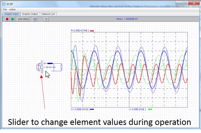
A distinct feature of the program is the capability to change the values of elements during the execution by means of sliders and thus the users get
an interactive lab type experience. This is a perfect tool for training mainly in the field of electronics, power electronics and electric power systems.
The program is unbelievably fast.
The author is constantly working on adding elements as well as more features in order to further improve the amazing user experience with the software.
There is a high-performance transient simulator version for free and registered members get access to a pro-version with much higher functionality including
for example 3-phase system simulation and frequency domain calculations. More to be discovered...
On a personal note: I am not aware of any other program running on a browser with this kind of performance it seems to be unique. I have invested a lot of
my free time in developing and testing the software. Should there still be bugs, please drop me a mail, I'll fix it as soon as possible.
I wish you dear customer lots of fun and satisfaction with this fantastic tool.
1.Introduction
The Electric Circuit Simulation Program ECSP is a numeric
simulator in the time and frequency domain for electric circuits. The time
domain simulator is based on well known differential equation linearization
techniques. The Gaussian Elimination allows an effective solution of linearized
equations. Similar techniques are used in most known programs such as EMTP, ATP
and Spice.
ECSP developers have focused on user friendliness and quick
response and less on accuracy of the used models.
ECSP allows a quick and easy positioning and connection of
elements as well as user friendly input of the element parameters.
Unique features of ESCP are the browser start and the possibility
to change elements during the execution by means of sliders popping up on elements.
There is a public simulator with a time domain version of the software.
The members area is accessibly for a yearly fee, to cover the development costs. In the members area
the simulator provides a higher functionality, see the description in the home page.
online circuit simulator
2.Prerequisite
ECSP has been tested for and runs on most common bowsers except IE (will apparently be deprected).
The best user experience however is possible with Google Chrome, followed by Firefox and Opera.
IMPORTANT:
Enable JavaScript on your browser (see the related browser specific links).
Do not delete browser history: ECSP stores the circuit you are working on in the browser storage, therefore do not delete the browser history for this specific program
(make an exception on your browser, see related browser specific links).
If you or the browser setting delete the history, you loose the circuit every time you close the browser window, otherwise the circuit is reloaded
automatically when you open the same browser again later.
No other data are stored on the browser or uploaded for any purpose what so ever
3.Build a circuit
Select a new element
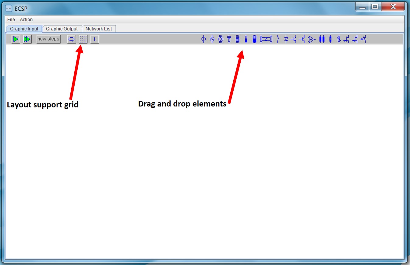
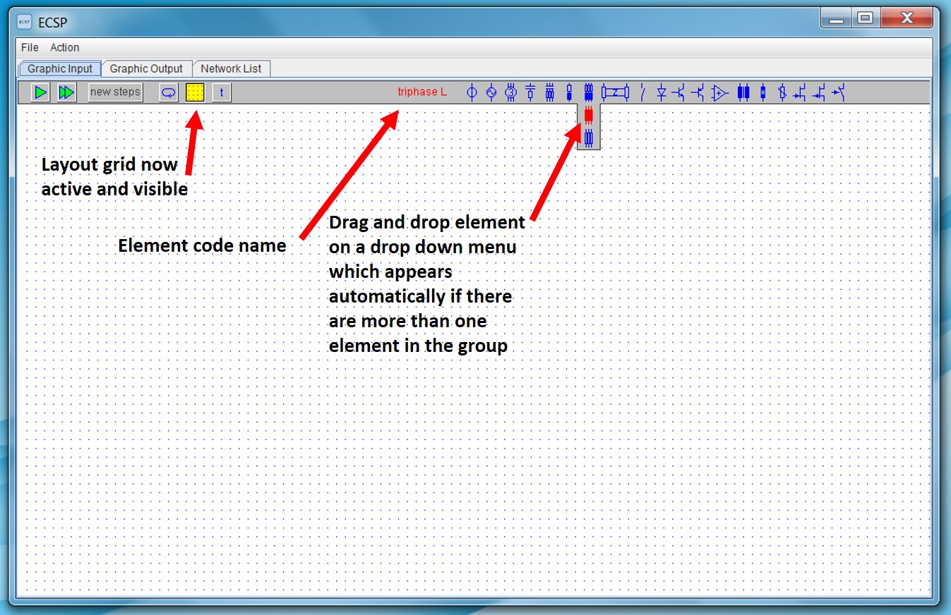
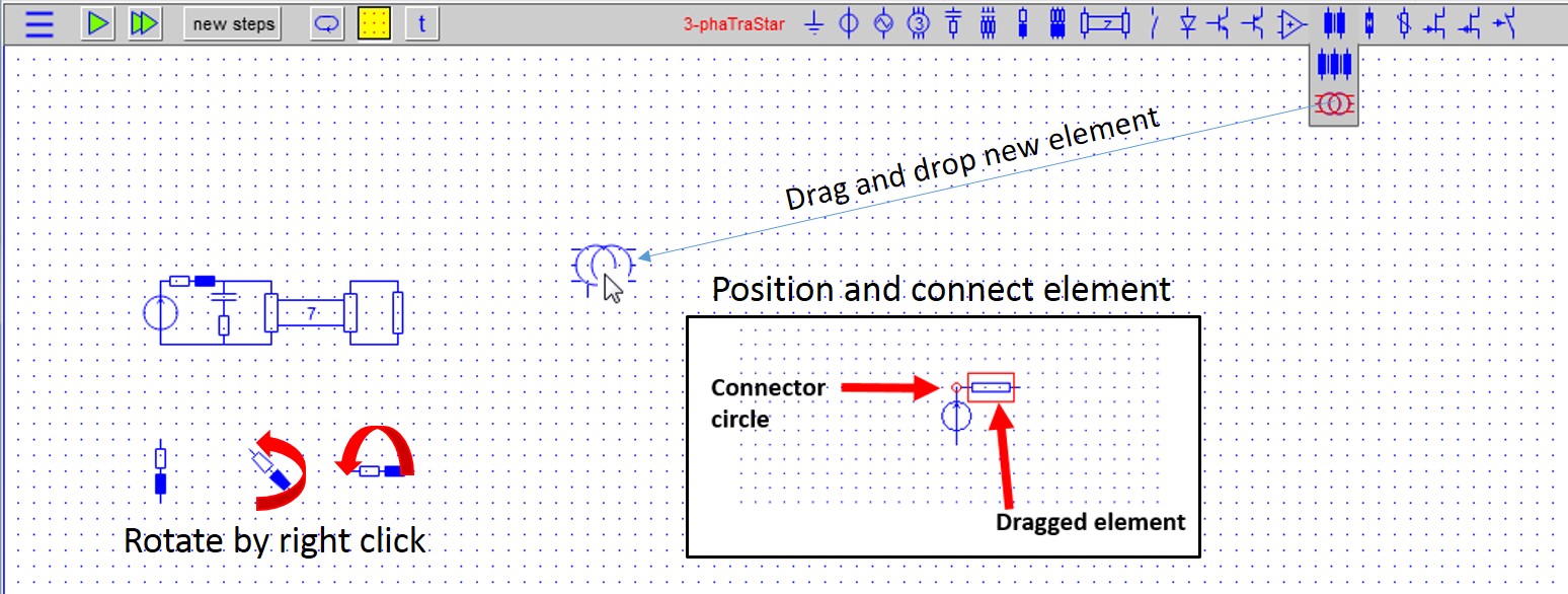
Activate layout support grid option for aligned positioning of elements (the white screen gets a dotted structure which attracts the element connectors).
Select an element on the element-selection menus.
The elements are grouped and many elements will appear in a pull-down menu on mouseover.
The element type selected appears in red on the selection bar.
By drag&drop the element is automatically added to the element list and will stay on the screen.
online circuit simulator
4.Add new elements or delete existing elements
Drag and drop the selected element anywhere on the screen. This automatically adds the element to the network list.
Elements can be dropped down to the canvas initially without any order and they can be re-positioned and connected later (see next).
Delete an existing element: Mousover it in order to highlight it and press DELETE.
An element can be deleted from inside the element parameters input form as well (see later).
online circuit simulator
5.Position elements
Move and position the element on the screen by drag and drop.
If the connector of an element comes close to another element, a red circle will appear and the element will snap with mouseup.
In this way the element is already connected to the neighbor.
Elements not connected directly will be connected by lines (see later).
If the layout grid is active, the elements will snap to the grid as long as it does not snap to another element, for a cleaner layout.
Change the orientation of the element by mouse right-click. Each right click turns the element by 450.
online circuit simulator
6.Connect elements
Elements can be connected directly or by lines.
If the connector of a dragged element comes close to another element, a red circle will appear and the element will snap with mouseup.
In this way the element is already connected to the neighbour.
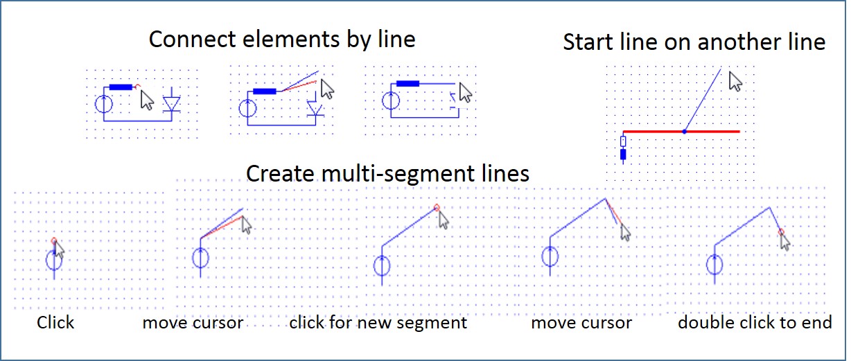
Elements not connected directly will be connected by lines:
Put the cursor on the connector of an element and the attractor (red circle) will appear
Click the left mouse button and move the mouse without button pressed. The line will appear between the starting point on the connector and the mouse.
(A new connecting line can only be started at a connector of an element or of a line or from anywhere on an existing line segment).
Click the mouse at the target connector of another element, the two element connectors are now connected via the line.
For a line ending blank: double click the left mouse button. You can connect an element to the open connecting line end later.
Lines can be segmented for flexibility. To break and change the direction of the line: left click and automatically the old line segment terminates
and a new line segment is attached (multi-line Fig. 6).
Multi segment lines will automatically adapt the line angles in order to get a cleaner circuit layout
Lines can start and end anywhere on an existing line.
Start a new line anywhere on double click.
Lines started unintentionally can be skipped by ECSP or Delete button.
online circuit simulator
7.Delete connection lines
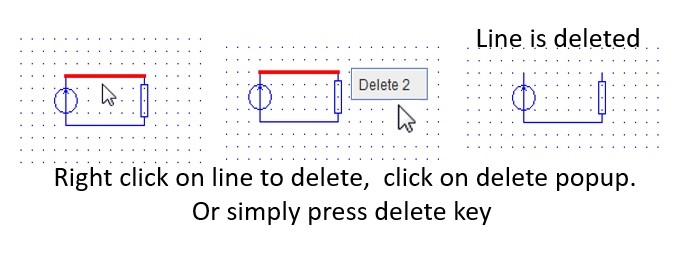
Touch the line with the cursor, it is highlighted
Push the DELETE key or right-click the line and delete it by clicking the delete popup.
Delete a group of lines by dragging a red rectangle over the lines to delete (see later).
online circuit simulator
8.Move a group of elements
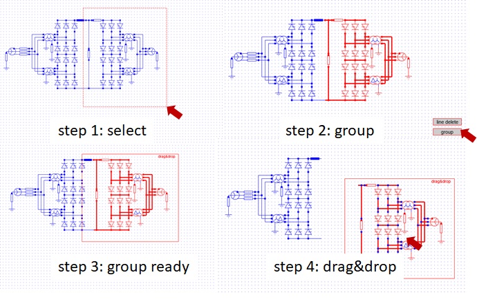
Start the drag in an empty space.
Drag the rectangle until all elements to be moved are inside the rectangle.
Push the group popup button or the delete lines button (for deleting the lines only.).
If the group button is confirmed, a rectangle will appear around the group. It can be drag&dropped to a new location on the screen.
Leave the move mode by clicking outside the red rectangle.
online circuit simulator
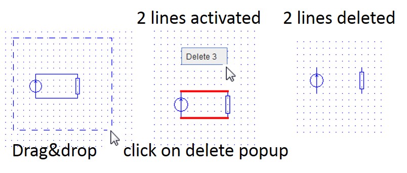
9.Remove several lines in one go
Delete a group of lines by dragging a red rectangle over the lines to delete.
Start the drag in an empty space.
Release the mouse and the lines inside the selection rectangle will be highlighted.
Delete by pushing the DELETE popup or click on empty space to undo selection.
online circuit simulator
10.Build 2 or more completely independent circuits running in parallel
It is possible to build two independent circuits without any connection in between
online circuit simulator
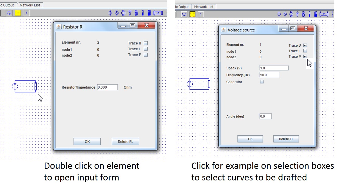
11.Input element parameters
Touch the element with the mouse (the element is highlighted by a red rectangle).
Double-click the element.
The menu for the selected element opens as popup:
Most elements need inputs (exceptions will be shown later). On the top right side tick the element curves you want to see: U (voltage), I (current), P (power).
Confirm with OK or delete the element.
Double-click the element.
online circuit simulator
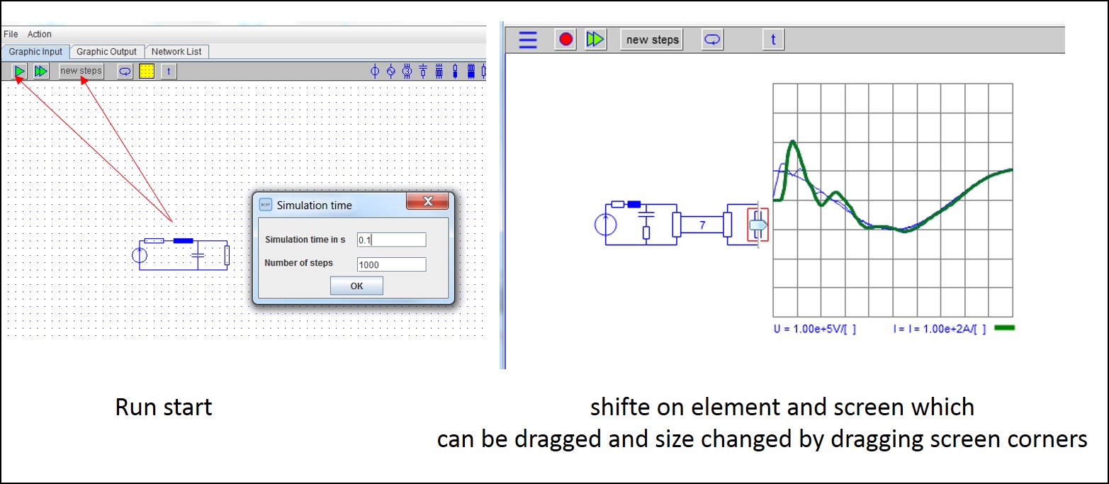
12.Run simulation
Run the simulation, once all element parameters are correctly entered as follows:
Click on new steps for the first run or on the green single triangle. For the first run, the simulation time set window opens automatically and suggests a time and step number based on an estimation.
Enter the simulation time and the number of steps to be performed. The number of steps should be so high that the individual time steps are shorter
than the period of the highest frequency possible in the circuit. The more time steps, the higher the accuracy will be.
Press OK and wait until the curves appear on the screen (the green arrow will be replaced by a red dot (simulation mode is active):
To stop the simulation mode, press on the red dot, the green arrow will appear again.
As long as the simulation mode is on (red dot), sliders popup on elements when touched. The element values can be changed by moving the slider up and down. after any change of the slider position, the calculation restarts.
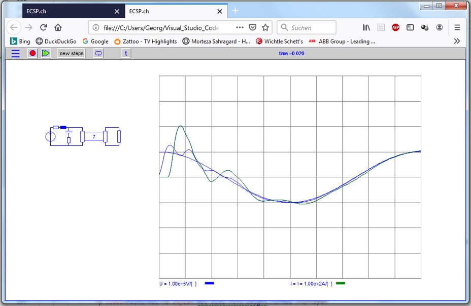
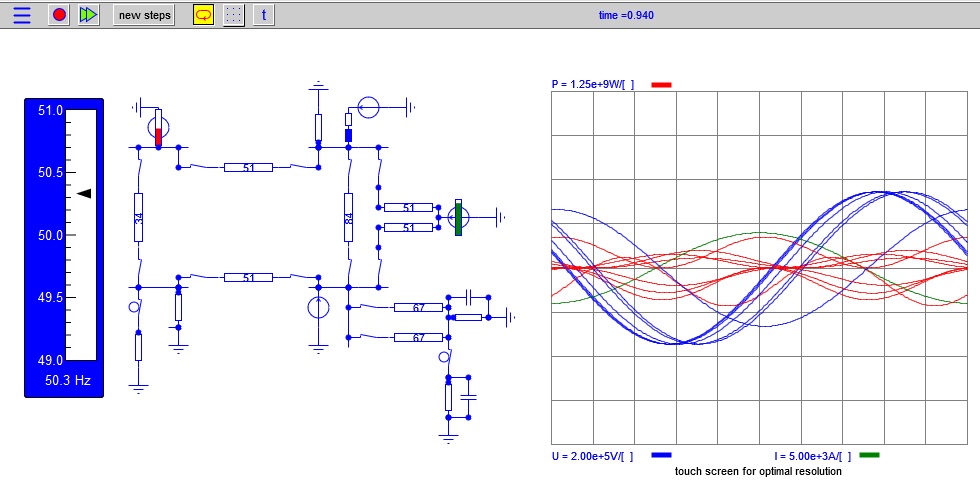
The result of the simulation is directly shown in the oscilloscope on the canvas. All the curves selected in the element parameters are displayed.
The green curves represent currents.
The blue curves represent voltages.
The red curves represent power.
The resolution of the curves are shown around the oscilloscope.
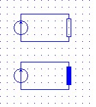
If you touch an element during simulation, the corresponding trace in the oscilloscope will be highlighted
You can move around the oscilloscope by drag&drop.
You can change the size of the oscilloscope by drag&drop of the corners (red dots appear when mousover a corner)
In the simulation mode, changes in the circuit topology are disabled.
online circuit simulator
13.Continue the simulation for another time span
By pressing on the double arrow, you can continue the simulation for another time span without restarting from the initial conditions.
You can change the simulation time and resolution of the next span before clicking the double arrow. So you can slowly approach a critical event.
online circuit simulator
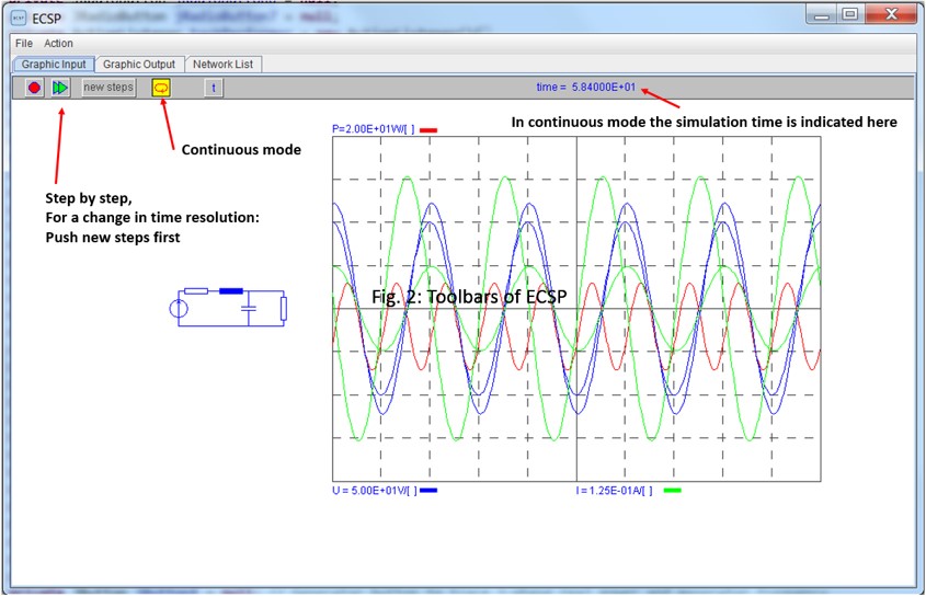
14.Simulation in continuous mode
Press the loop symbol for continuous simulation. The speed of the simulation depends on the size of the network and the time resolution.
The simulation time is indicated in the tool bar.
In order to get a synchronized picture, the simulation time should correspond to a multiple of the lowest source frequency cycle
available in the network. The program makes a suggestion.
online circuit simulator
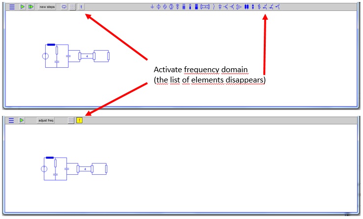
15.Simulation in frequency domain 1 of 2
The t-domain and f-domain button switches between the time domain and the frequency domain simulator.
When pressing the f-domain button, the program asks for input of the lowest and highest frequency to be calculated.
Build the circuit and run it first in the normal time domain mode (t button). This first t-domain run is especially important to adjust operating
points of non-linear elements such as transistors and copy it into the frequency domain mode.
The circuit cannot be built in the frequency domain mode. In order to change the circuit layout, add or delete elements, switch to the t-domain.
In the f-domain, the list of drop down elements is not visible.
Some non-linear elements such as non-linear inductors or arrestors are not available in the f-domain, replace them by linear elements.
online circuit simulator
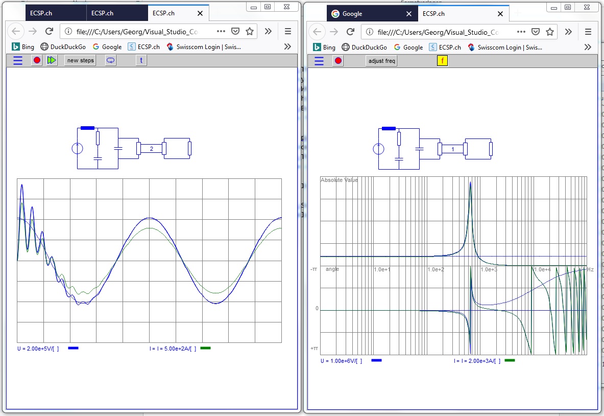
16.Simulation in frequency domain 2 of 2
The frequency domain trace screen (to the right) is subdivided in an amplitude segment, on the upper half of the graph and in a phase angle segment at the bottom.
The phase angle graph varies between + and - Pi.
The value of most elements can be varied during the simulation by means of sliders appearing when the mouse hits the element, except some such as sources.
For changes in the topology or adding / deleting elements, please switch to the t-domain.
online circuit simulator
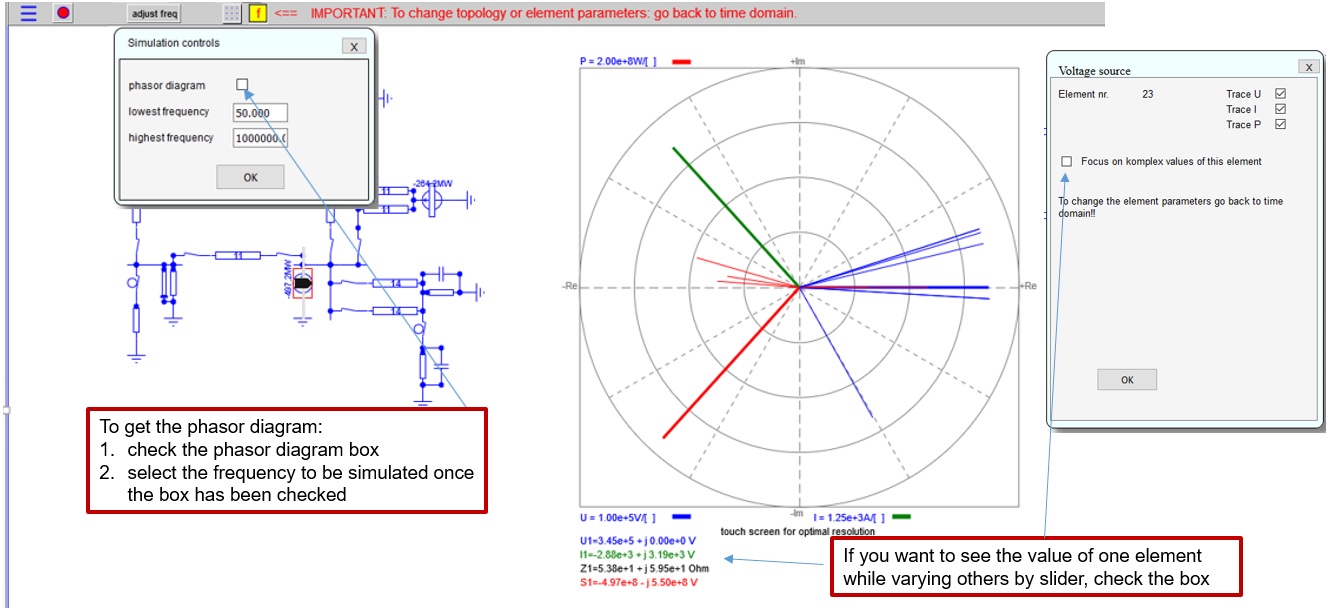
17.Simulation as phasor diagrams
The traces are represented as phasors in Re and Img diagram.
Get to this mode by:
1. switching to the frequency domain
2. checking the phasor diagram box in the adjust frequency button .
3. selectring the frequency to be simulated (i.e.: 50 Hz).
The value of most elements can be varied during the simulation by means of sliders appearing when the mouse hits the element, except some such as sources.
For changes in the topology or adding / deleting elements, please switch to the t-domain.
Individual traces of the elements however can be check in or out in this mode.
online circuit simulator
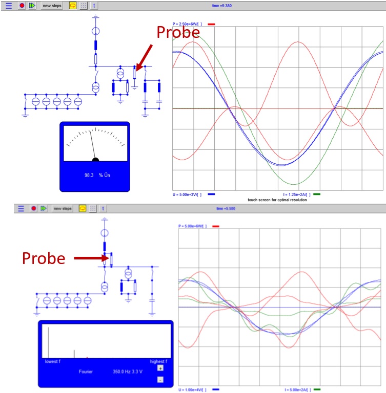
18.Show vuMeter with uPeak or Fourier analysis of a trace
Drag and drop the probe element under the earth sign just like a resistor.
Double click
For vuMeter: Enter the Voltage which shall be 100% peak value (i.e. Unominal peak). Run in continuous mode
For Fourier analysis: check the box.
Fourier analysis can be made for voltage or for current if probe is parallel to a shunt resistor.
online circuit simulator
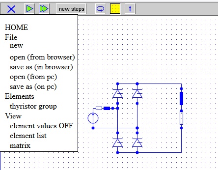
19.Menu items
Home
New network
Local network file storage on browser (open old file, store new file, delete existing file)
Local network file storage on pc (open old file, store new file, delete existing file
Trigger control for thyristor groups
Show element values
Show elements list of the network
online circuit simulator
20.Menu items
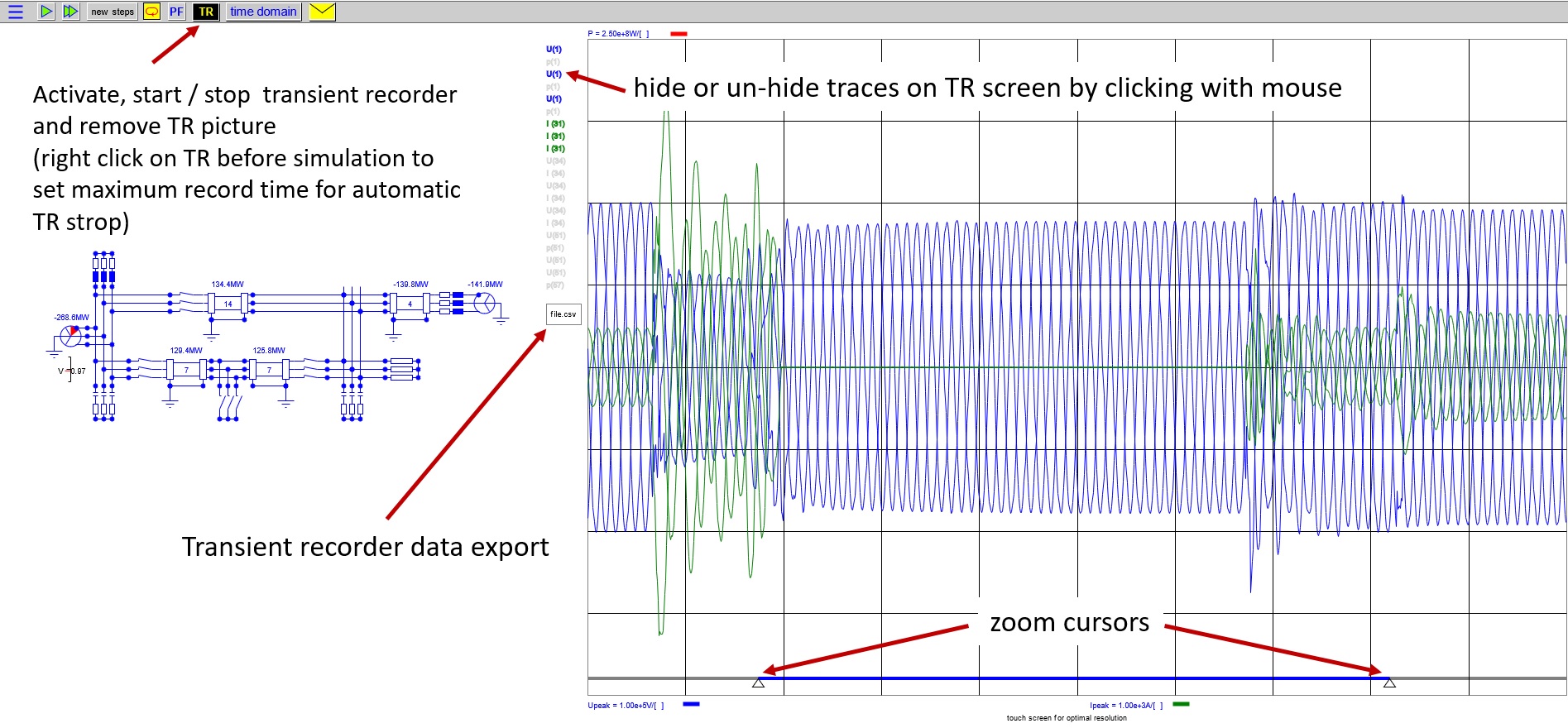
The transient recorder function is available for the time domain.
TR can be activated only if "continuous" is set<./li>
When TR is active it blinks.
Recording of traces starts as soon as the simulation runs in continuous mode, active TR provided.
The transient recorder function shows the simulation traces from the instant TR is activated until it is clicked again or the simulation is stopped.
Instead of having to stop the recording manually, the maximum length of the record can be set as long as TR is inactive by right-clicking on TR.
To show the record click the blinking TR or click the red/black blinking run/stop buton at the top left.
With TR active before the start the simulation, the recording starts at the beginning of the simulation.
TR activeed after the start the simulation, the recording starts after simulation start at the moment of TR click.
Switches in O-C mode can be trggered by the TR start if the corresponding box on the switch is clicked.
On the TR screen the 2 cursors at the bottom enable zooming.
The list of the traces to the left of the screen enables hiding of the traces which are of no interest by clicking on them.
If the mouse touches a trace, the value of the trace is shown as and the corresponding element on the circuit is highlighted by a red square.
IMPORTANT: You can activate TR after the start of the simulation, so you can adjust the network conditions before recording starts by pressing TR. Thus you can watch a load rejection out of full load condition.
Recorded traces of the transient recorder can be exported to csv files for reuse in programs such as excel..
online circuit simulator
21.Menu items
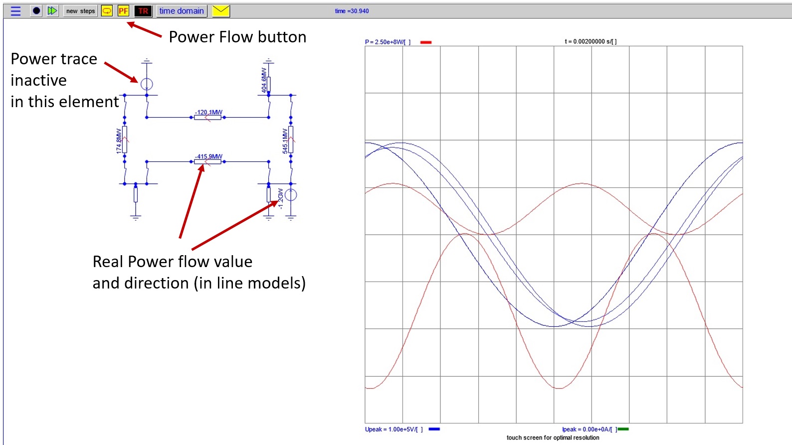
The "PF" button on the control/command stripe marks the real power flow values on elements while the simulation runs.
Active "PF" button (yellow) shows real-power indicators on U sources, R and lines even when the power trace tick-box in the element input mask is un-ticked.
Purpose: the number of traces in the screen can be reduced without loosing the power flow information.
"PF" can be activated only in mode "time domain" and in mode "phasor app"
online circuit simulator
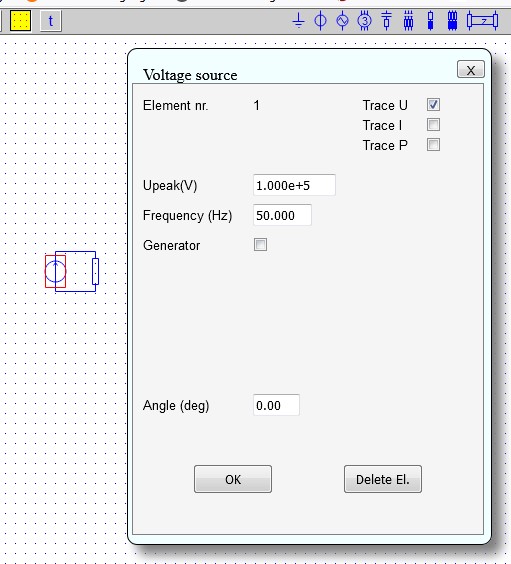
1.Voltage source single phase
The voltage source simulates a sinusoidal source voltage oscillating with selectable frequency.
Other sources available :
Current source
DC source (+/-)
Triangular saw tooth
The angle input field establishes an angular shift of the start angle of the source voltage.
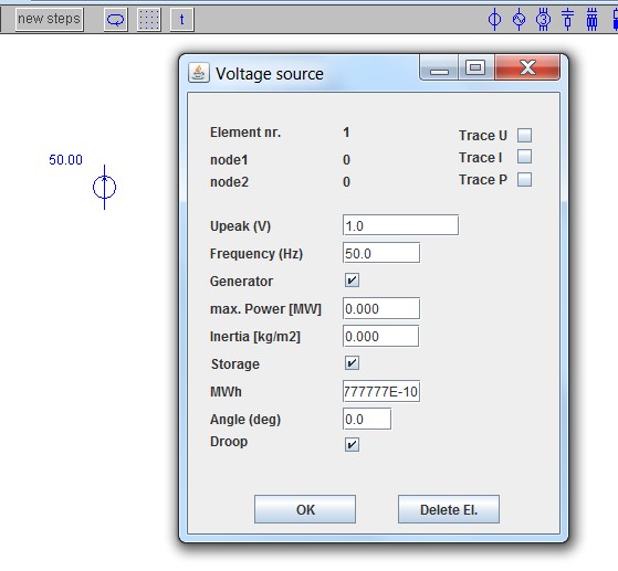
2.Voltage source Power Generator
By clicking the Generator box, the voltage source is transformed to a Power Generator with rotating mass
The power output of the Generator is controlled by the momentum applied to the Generator during the simulation and by the load
The momentum is controlled by a shifter on the generator during the simulation
The maximum power can be set in the input box
Recommended inertia: 150 – 250 kg/m2/MW. Setting a realistic inertia is mandatory in order to avoid uncontrolled oscillation. The model is realistic.
The “Droop” checkbox enables to stabilize the frequency around the generator nominal frequency entered in the frequency input field. The droop supports oscillation damping.
The principle of a droop is well explained in various internet links. A droop is a controller which reduces the mechanical input power of the generator if the frequency
exceeds the nominal frequency and increases the mechanical input power in case the frequency falls below nominal.
The output power of the generator is the sum of the mechanical torque and the change in spinning energy.
With the storage checkbox on, an energy storage unit can be simulated.
Input: the storage capacity.
.
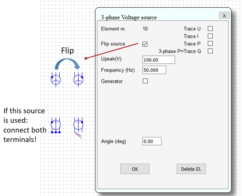
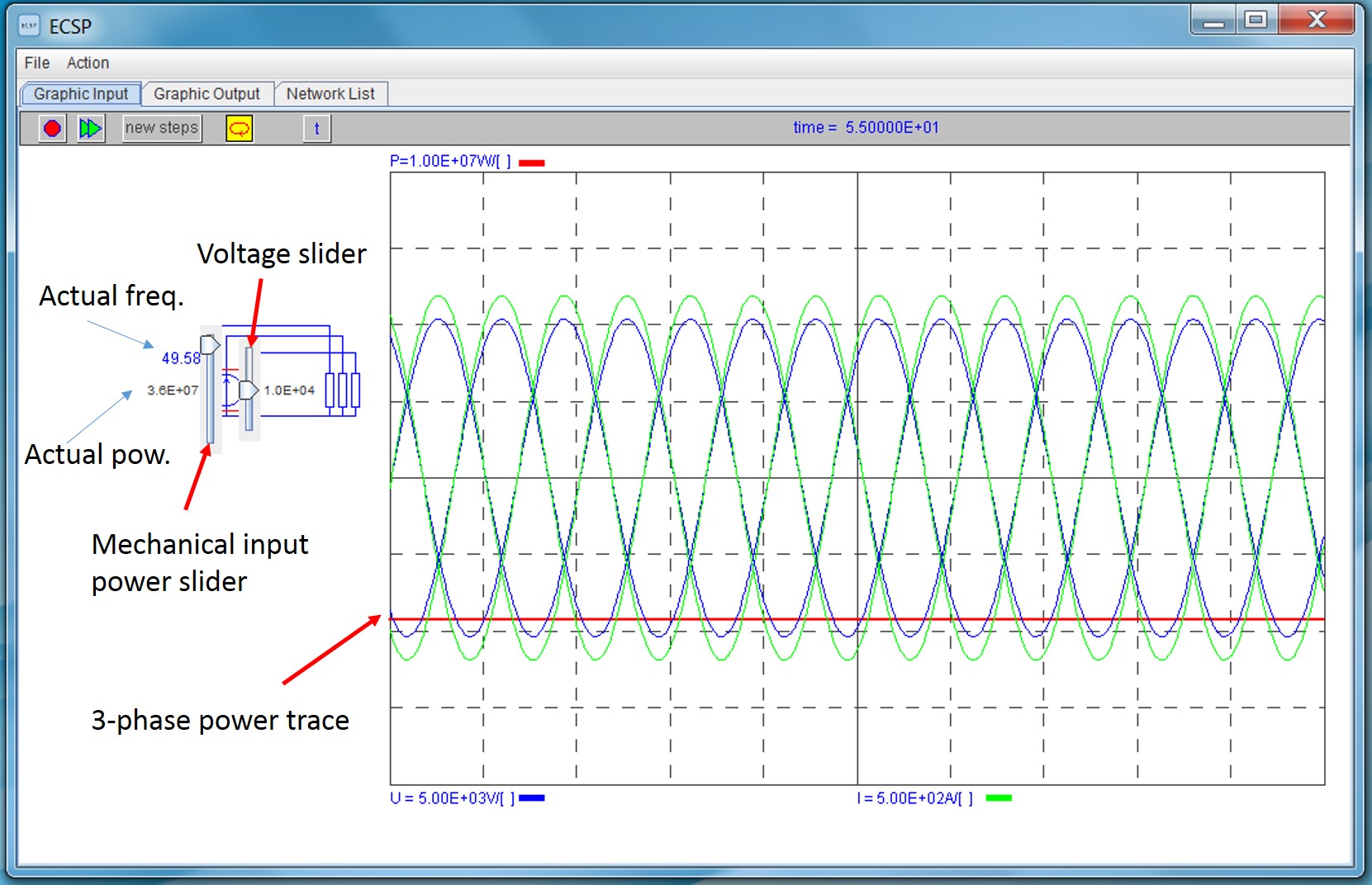
3.3-phase voltage source
As for the single phase voltage source, the 3-phase source operates as a source or as a generator in case the related check-boxes are activated. The 2 differences:
A 3-phase power trace G can be recorded and traced instead of a separate power trace for each individual phase. The 3-phase power trace calculates the sum of the real power of the 3 separate phases and the sum of the reactive power of the 3 phases will be zero in case of a balanced system. The 3-phase power trace will be a straight line in case of a balanced system.
The 3 phase system should be grounded on one end, i.e., the 3 connectors at one end of the generator should be interconnected by means of a connecting line to form the star point of the generator or use the source already grounded. The connector with a dot represents phase R. Phases S is delayed by 120 electrical degrees and phase T by 240 deg.
When connecting several 3-phasse units to one system, make sure that the right phases are connected with each other, otherwise the result will be meaningless.
4.3-phase Power Generator
The picture below illustrates the features of a 3-phase Power Generation simulation with the 3-phase active power output trace in red.
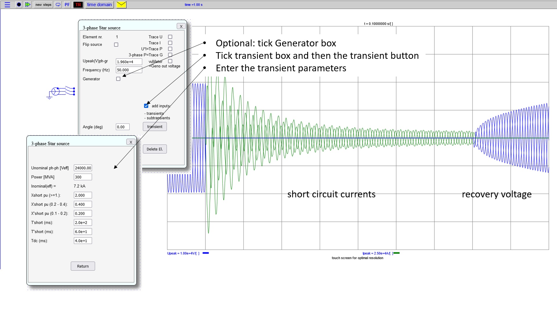
4.3-phase Generator transient shortcircuit model
Double click the 3-phase voltage source
Check or un-check the generator tick box
Generator box checked: Behaves as a true geno with automatic adjustment of rotor angle depending on power supply
Generator box un-checked: Behaves as a voltage source with static frequency but with manually adjusted rotor angle
IMPORTANT: the voltage input will be performed in the transient mask and will be taken over automatically
Check the "add inputs" checkbox
Press the transient button
Enter the data in the transient entry mask
The nominal voltage is 3-phase rms (IMPORTANT: the single phase peak value in the main mask is automatically adjusted)
Press "enter" after every input
None of the values shall be zero!
Press the "return" button
With vuMeter box ticked you will see the rotor angle and the output voltage indicator during simulation
The nominal voltage tays static during simulation, the peak-phase-ground voltage however can be adjusted by sliders during the simulation
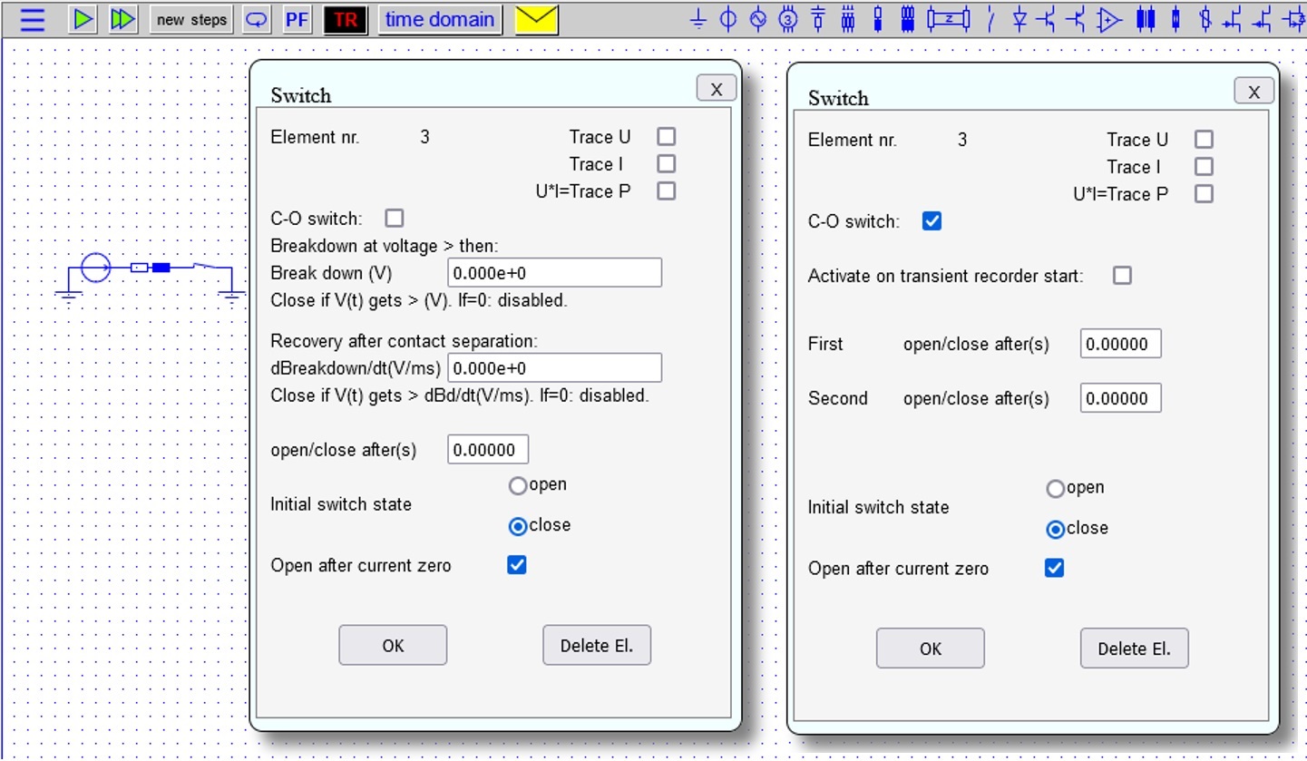
5.Switches for 1- and 3-phase circuits
Basic switch with one opening or one closing operation (C-O box un-ticked)
C-O box ticked: For a 2-operation breaker with 2 distinct operation times
The C-O timer can be triggered by starting the transient recorder, provided the corresponding box is checked.
Switches to open and close xyz seconds after simulation start
Option: current interruption after current zero
Option: initial state open or close
Option: close on overvoltage
Option: break down voltage in function of contact travel
Switch with random open and close function
Manual operation if time is set <= 0
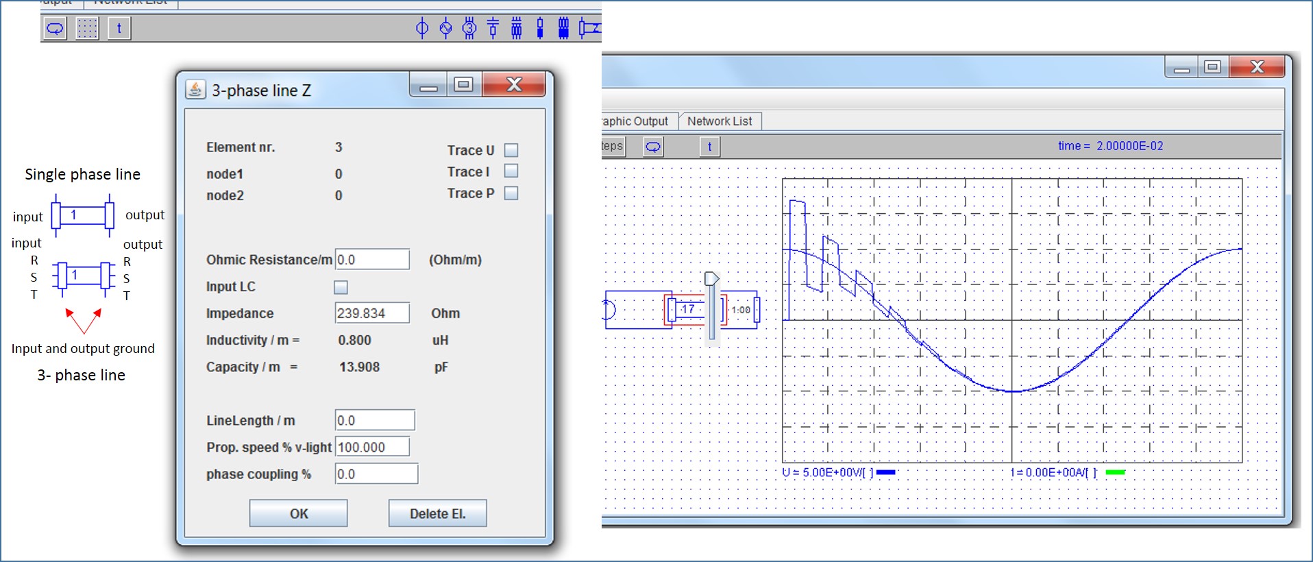
6.Long line (1- and 3-phase)
The long line simulates a bi-directional traveling wave.
It is a typical line segment register model.
The number of segments is proportional to the speed of the wave on the line divided by the time step. It calculates a superposition of the forward and backward moving wave.
The input of the surge impedance is either by input of the Z-impedance in Ohm or alternatively by input of the inductance and capacitance per meter.
The alternative input mode can be selected. Both modes are equivalent
All other inputs are self evident.
For a 3-phase system, there is a optional input for the phase coupling in %.
The earth connection of the 3-phase line is the bottom connector on both line ends.
During simulation a slider appears when the cursor hits the line. The slider enables smoothening the result a bit, it decreases the rate of rise (e.g. like adding a small capacitor at
the entrance). It is useful when performing complex simulations resulting in high frequency transients on the line which in reality would be damped a bit
7.Grounded power flow line
Same model as the long line but with integrated grounding.
Therefore at least one other element must be grounded, best ground a source or all sources.
All the rest is equal to the model described above.
online circuit simulator
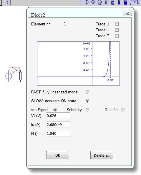
8.Diode
The diode is based on a fast fully linearized model or, alternatively on an accurate but a little slower (recommended) model.
The accurate model is well described in literature.
3 pre-set basic settings can be selected, small signal, Schottky or rectifier.
More diode characteristics can be set by choosing appropriate values in the Slow but accurate model.
The difference between the accurate model and the fully linearized model are visualized in the parameter input window.
Id = Is * (e (Ud/(N*Vt)) - 1)
N = 1..2
Vt ≈ 26 mV
Is ≈ 10 -12 … 10 -6 A
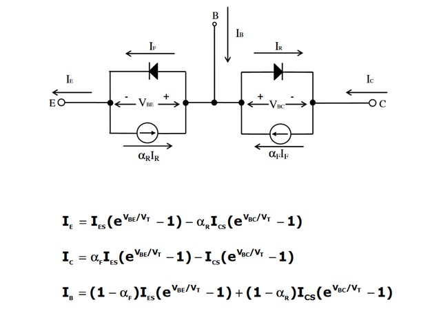
9.Bipolar transistor
The bipolar transistor is modeled according to the Ebers-Moll model (see internet) of a bipolar transistor.
In the transistor input mask Bbc = αF and Bbe = αR.
Vtbe, Isbe, Vtbc and Isbc represent the diode values already shown in the diode model above. The multiplier N is not used and assumed 1.
The screen in the input mask demonstrates the model.
For the frequency domain model, the slider should be set to the expected bc voltage in order to get the right input resistance.
Alternatively a pre-run in the time domain should be performed in order to get the exact value for the input resistance automatically.
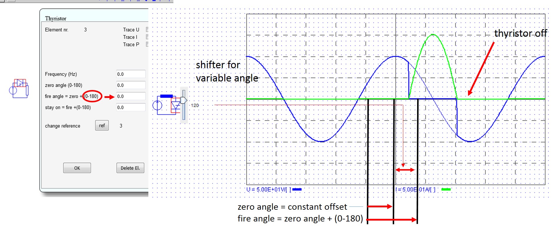
10.Thyristor
The Thyristor fires when reaching the firing angle. The Thyristor closes when the current crosses zero again.
The starting point is the positive zero crossing of the voltage across the Thyristor or, alternatively, the voltage from a reference voltage source.
Normally it is better to use a reference, since the voltage across the Thyristor may be disturbed
Frequency: The reference frequency is needed to transform the firing angle into time delay, i.e. form for example at 50 Hz from 90o to 5 ms delay after zero crossing of the reference.
Reference:The default reference is the Thyristor voltage. By pushing on the ref button, an external 1-phase voltage reference can be indicated as clock maker. The number appearing after pushing on the reference source is the element number of the reference source.
In case an element is deleted or added, the reference numbers of all Thyristors should be revisited.
Zero angle (0-180):This is a firing delay offset angle added to the variable firing angle. Normally the zero angle can be left 0. It is for example used when various Thyristors operating on different phase use the same reference source or when one Thyristor shall fire on the negative sequence.
Fire Angle>:This is the variable angle added to the offset. This one can be controlled by the slider during the simulation.
Stay on:Switching off after firing is suppressed for the angle entered here in order to avoid the thyristor to switch of during high frequency current oscillations after firing.
Build control groups:Bild a common group of thyristors controlled simulataneously: Explained above under the Menu item 18.
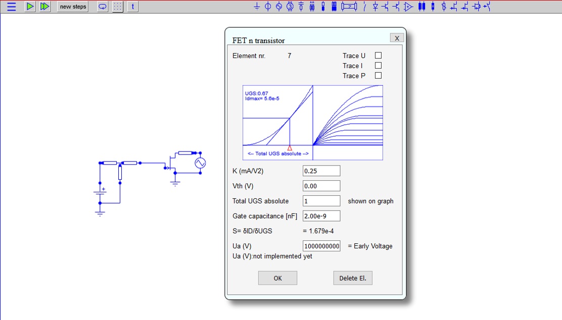
11.Fet transistor
Description see video above.
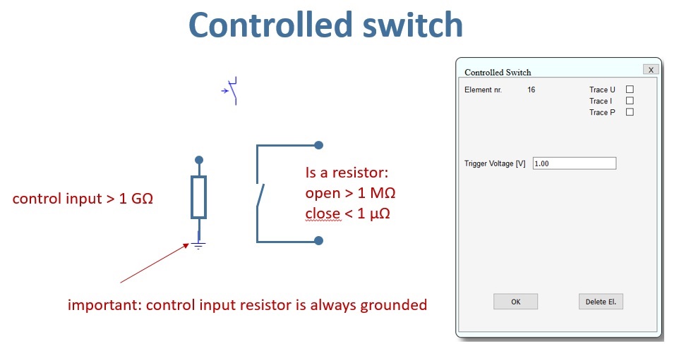
12.Controlled switch circuit
The controlled switch opening and closing is controlled by the gate voltage.
long as the gate voltage is >= the trigger voltage entered in the field.
Important: The input resistance of the gate is always grounded. You need a second eart element and another object.
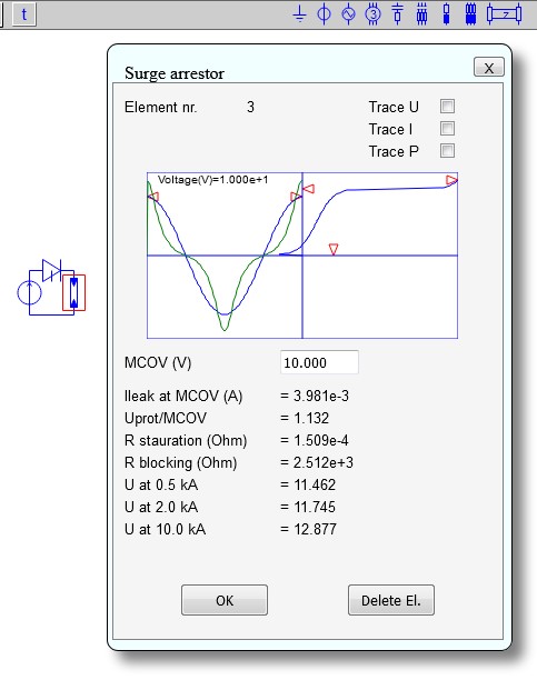
13.Surge arrestor
The element models a typical Metal Oxide varistor, i.e.: surge arrestor.
Set the maximum continuous operating voltage (normally around 10 – 15% higher than the nominal operating voltage).
By moving the voltage cursor you can set the characteristics and check the impact of the applied voltage on the arrestor current.
You can set the protection voltage level by varying the cursor to the right of the center line.
Play around with the individual currents in order to understand the impact of the individual parameters on the arrestor characteristics.
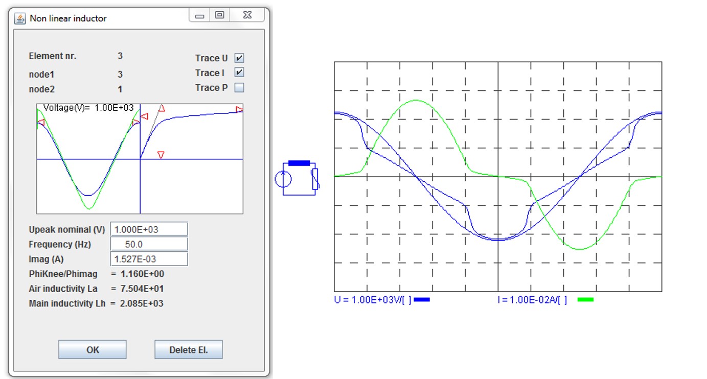
14.Inductivity with saturation
Procedure to set-up the non-linear inductivity:
Enter the Upeak nominal, the base frequency and the expected magnetization current at U nominal.
The non-linear characteristics of the Flux (phi) is represented by the curve on the right hand side.
Fine tune the characteristics by shifting the red setting triangles (cursors) as follows (the name of the setting cursor appears as soon as it is hit by the mouse):
The phi Nominal cursor sets the magnetization flux at Upeak nominal.
The magnetization current cursor sets the magnetization current at phi Nominal
The Phi knee cursor sets the knee point of the flux relative to the Phi Nominal (= Phimag). It must be > Phi Nominal.
The Linear part of Magnetization current cursor sets the smoothness on thee way to saturation.
The Phi saturation cursor sets the flux of the saturated inductivity (air core reactance).
Playing with the applied voltage cursor simulates the behavior of the current through the non-linear inductor (green curve) assuming a sinusoidal source.
This cursor does not affect the characteristics of the inductivity.
Important remark: When opening the input mask, the shape of the curve is re-adjusted in order to get best visibility of the characteristics. The data entered and stored previously remain unchanged.
This may be a little confusing in the beginning.
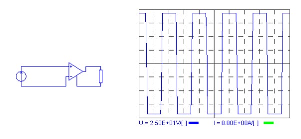
15.Operational Amplifier and Comparator
The operational amplifier can be operated with a saturation corresponding to the supply voltage.
The operational amplifier can work as a comparator.
Table of content
GoTo user's Guide.pdf paper
Introduction
Prerequisite
Build a circuit
Add new or delete element
Position elements
Connect elements
Delete connection lines
Move a group of elements
Remove several lines in one go
Build 2 or more independent circuits
Input element parameters and curves to be shown
Run simulation
Continue simulation
Continuous mode
Frequency domain 1
Frequency domain 2
Phasor diagram
Volt meter and Fourier analysis
Menu
Transient Recorder
PowerFlow PF button
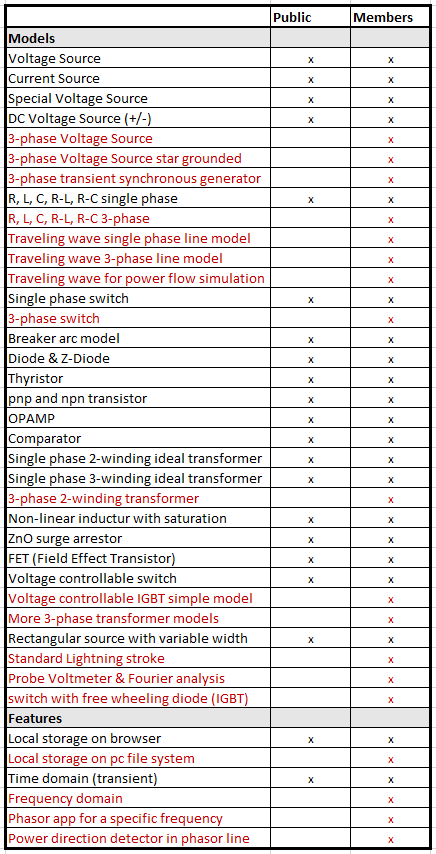
list of elements (not all listed)
Voltage source single phase
Voltage source Power Generator
3-phase voltage source
3-phase Power Generator
3-phase Generator transient shortcircuit model
Switches for single and 3-phase circuits
Long line (1- and 3-phase)
Grounded Long line (1-phase) for single phase power flow analysis